Table of Contents
Running the Solver xspecfem3D
Now that you have successfully run the mesher, you are ready to compile the solver. For reasons of speed, the solver uses static memory allocation. Therefore it needs to be recompiled (type ‘make clean’ and ‘make specfem3D’) every time one reruns the mesher with different parameters. To compile the solver one needs a file generated by the mesher in the directory OUTPUT_FILES called values_from_mesher.h, which contains parameters describing the static size of the arrays as well as the setting of certain flags.
The solver needs three input files in the DATA directory to run: the Par_file that was discussed in detail in Chapter [cha:Running-the-Mesher], the earthquake source parameter file CMTSOLUTION or the force source parameter file FORCESOLUTION, and the stations file STATIONS. Most parameters in the Par_file should be set prior to running the mesher. Only the following parameters may be changed after running the mesher:
-
the simulation type control parameters:
SIMULATION_TYPEandSAVE_FORWARD -
the record length
RECORD_LENGTH_IN_MINUTES -
the movie control parameters
MOVIE_SURFACE,MOVIE_VOLUME, andNTSTEPS_BETWEEN_FRAMES -
the multi-stage simulation parameters
NUMBER_OF_RUNSandNUMBER_OF_THIS_RUN -
the output information parameters
NTSTEP_BETWEEN_OUTPUT_INFO,NTSTEP_BETWEEN_OUTPUT_SEISMOS,OUTPUT_SEISMOS_ASCII_TEXT,OUTPUT_SEISMOS_SAC_ALPHANUM,OUTPUT_SEISMOS_SAC_BINARYandROTATE_SEISMOGRAMS_RT -
the
RECEIVERS_CAN_BE_BURIEDandPRINT_SOURCE_TIME_FUNCTIONflags -
the
USE_MONOCHROMATIC_CMT_SOURCEflag
Any other change to the Par_file implies rerunning both the mesher and the solver.
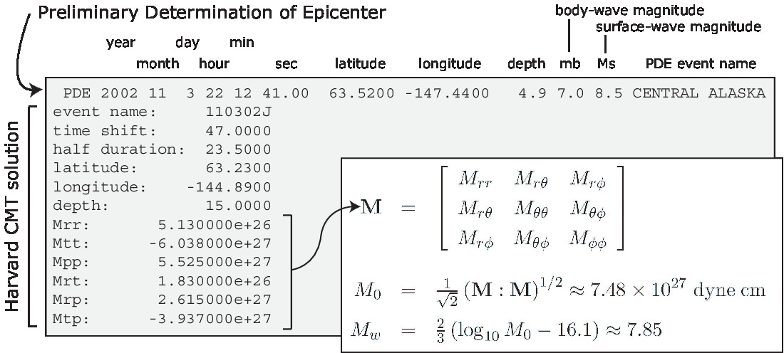
For any particular earthquake, the CMTSOLUTION file that represents the point source may be obtained directly from the Global Centroid-Moment Tensor (CMT) web page. It looks like this:
The CMTSOLUTION should be edited in the following way:
-
For point-source simulations (see finite sources, page ), setting the source half-duration parameter
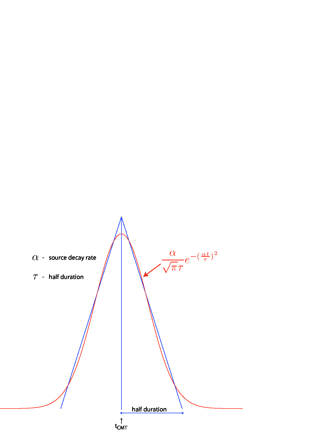
half durationequal to zero corresponds to simulating a step source-time function (Heaviside), i.e., to using a moment-rate function that is a delta function. Ifhalf durationis not set to zero, the code will use a smooth (pseudo) Heaviside source-time function with a corresponding Gaussian moment-rate function (i.e., a signal with a shape similar to a ‘smoothed triangle’, as explained in Komatitsch and Tromp (2002) and shown in Fig 1.2) with half-widthhalf duration.Often, it is preferable to run the solver with
half durationset to zero and convolve the resulting synthetic seismograms in post-processing after the run, because this way it is easy to use a variety of source-time functions (see Section [sec:Process-data-and-syn]). Komatitsch and Tromp (2002) determined that the noise generated in the simulation by using a step source time function may be safely filtered out afterward based upon a convolution with the desired source-time function and/or low-pass filtering. Use the postprocessing scriptprocess_syn.pl(see Section [sub:process_syn.pl]) with the-hflag, or the serial codeconvolve_source_timefunction.f90and the scriptutils/convolve_source_timefunction.cshfor this purpose, or alternatively use signal-processing software packages such as SAC. Typemake convolve_source_timefunctionto compile the code and then set the parameter
hdurinutils/convolve_source_timefunction.cshto the desired half-duration. -
To use a monochromatic source-time function instead, enable the flag
USE_MONOCHROMATIC_CMT_SOURCEinPar_file. In this case,half durationwill be interpreted as the period of the source-time function. By default, the left side of the source-time function is applied with a Hanning taper at a length of 200.0 s. This can be configured throughTAPER_MONOCHROMATIC_SOURCEinconstants.hfile. -
The zero time of the simulation corresponds to the center of the triangle/Gaussian, or the centroid time of the earthquake. The start time of the simulation is $t=-1.5*\texttt{half duration}$ (the 1.5 is to make sure the moment-rate function is very close to zero when starting the simulation. This avoids spurious high-frequency oscillations). To convert to absolute time $t_{\mathrm{abs}}$, set
$t_{\mathrm{abs}}=t_{\mathrm{pde}}+\texttt{time shift}+t_{\mathrm{synthetic}}$
where $t_{\mathrm{pde}}$ is the time given in the first line of the
CMTSOLUTION,time shiftis the corresponding value from the originalCMTSOLUTIONfile and $t_{\mathrm{synthetic}}$ is the time in the first column of the output seismogram.
If you know the earthquake source in strike/dip/rake format rather than in CMTSOLUTION format, use the C code utils/strike_dip_rake_to_CMTSOLUTION.c to convert it. The conversion formulas are given for instance in (Aki and Richards 1980). Note that the (Aki and Richards 1980) convention is slightly different from the Global/Harvard CMTSOLUTION convention (the sign of some components is different). The C code outputs both.
Centroid latitude and longitude should be provided in geographical coordinates. The code converts these coordinates to geocentric coordinates (Dahlen and Tromp 1998). Of course you may provide your own source representations by designing your own CMTSOLUTION file. Just make sure that the resulting file adheres to the Global/Harvard CMT conventions (see Appendix [cha:Reference-Frame-Convention]). Note that the first line in the CMTSOLUTION file is the Preliminary Determination of Earthquakes (PDE) solution performed by the USGS NEIC, which is used as a seed for the Global/Harvard CMT inversion. The PDE solution is based upon P waves and often gives the hypocenter of the earthquake, i.e., the rupture initiation point, whereas the CMT solution gives the ‘centroid location’, which is the location with dominant moment release. The PDE solution is not used by our software package but must be present anyway in the first line of the file.
In the current version of the code, the solver can run with a non-zero time shift in the CMTSOLUTION file. Thus one does not need to set time shift to zero as it was the case for previous versions of the code. time shift is only used for writing centroid time in the SAC headers (see Appendix [cha:SAC-headers]). CMT time is obtained by adding time shift to the PDE time given in the first line in the CMTSOLUTION file. Therefore it is recommended not to modify time shift to have the correct timing information in the SAC headers without any post-processing of seismograms.
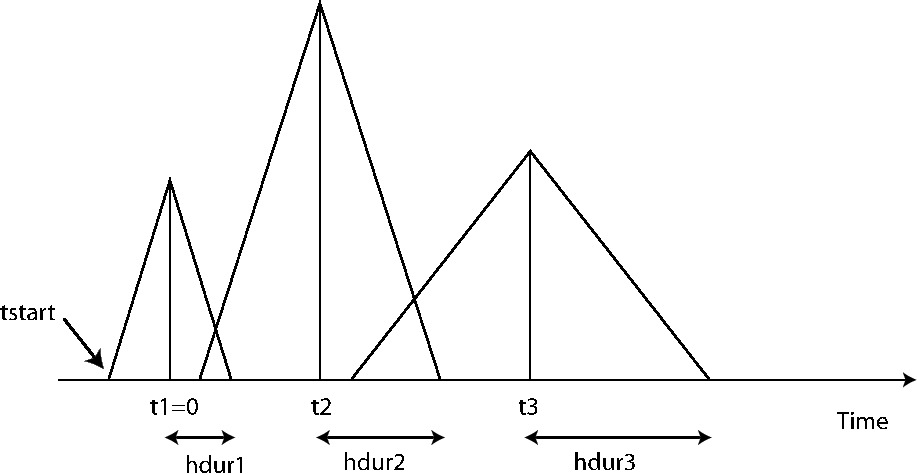
To simulate a kinematic rupture, i.e., a finite-source event, represented in terms of $N_{\mathrm{sources}}$ point sources, provide a CMTSOLUTION file that has $N_{\mathrm{sources}}$ entries, one for each subevent (i.e., concatenate $N_{\mathrm{sources}}$ CMTSOLUTION files to a single CMTSOLUTION file). At least one entry (not necessarily the first) must have a zero time shift, and all the other entries must have non-negative time shift. If none of the entries has a zero time shift in the CMTSOLUTION file, the smallest time shift is subtracted from all sources to initiate the simulation. Each subevent can have its own half duration, latitude, longitude, depth, and moment tensor (effectively, the local moment-density tensor).
Note that the zero in the synthetics does NOT represent the hypocentral time or centroid time in general, but the timing of the center of the source triangle with zero time shift (Fig 1.3).
Although it is convenient to think of each source as a triangle, in the simulation they are actually Gaussians (as they have better frequency characteristics). The relationship between the triangle and the Gaussian used is shown in Fig 1.2. For finite fault simulations it is usually not advisable to use a zero half duration and convolve afterwards, since the half duration is generally fixed by the finite fault model.
The FORCESOLUTION file should be edited in the following way:
-
The first line is only the header for the force solution, which can be used as the identifier for the force source.
-
time shift:For a single force source, set this parameter equal to $0.0$ (The solver will not run otherwise!); the time shift parameter would simply apply an overall time shift to the synthetics, something that can be done in the post-processing (see Section [sec:Process-data-and-syn]). -
half duration:Set the half duration value (s) for step source-time function. In case that the solver uses a (pseudo) Dirac delta source-time function to represent a force point source, a very short duration of five time steps is automatically set by default. For a Ricker source-time function, set the dominant frequency value (Hz). See the parametersource time function:below for source-time functions. -
latitude:Set the latitude of the force source. -
longitude:Set the longitude of the force source. -
depth:Set the depth of the force source (km). -
source time function:Set the type of source-time function: 0 = Gaussian function, 1 = Ricker function, 2 = Heaviside (step) function, 3 = monochromatic function, 4 = Gaussian function as defined in Meschede, Myhrvold, and Tromp (2011). -
factor force source:Set the magnitude of the force source (units in Newton N). -
component dir vect source E:Set the East component of a direction vector for the force source. Direction vector is not necessarily a unit vector. -
component dir vect source N:Set the North component of a direction vector for the force source. -
component dir vect source Z_up:Set the vertical component of a direction vector for the force source. Sign convention follows the positive upward direction.
Where necessary, set a FORCESOLUTION file in the same way you configure a CMTSOLUTION file with $N_{\mathrm{sources}}$ entries, one for each subevent (i.e., concatenate $N_{\mathrm{sources}}$ FORCESOLUTION files to a single FORCESOLUTION file). At least one entry (not necessarily the first) must have a zero time shift, and all the other entries must have non-negative time shift. Each subevent can have its own set of parameters latitude, longitude, depth, half duration, etc.
The solver can calculate seismograms at any number of stations for basically the same numerical cost, so the user is encouraged to include as many stations as conceivably useful in the STATIONS file, which looks like this:
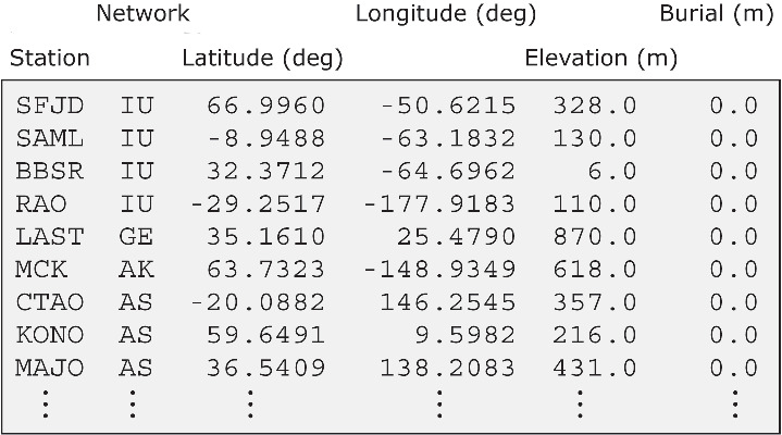
Each line represents one station in the following format:
Station Network Latitude(degrees) Longitude(degrees) Elevation(m) burial(m)
If you want to put a station on the ocean floor, just set elevation and burial depth in the STATIONS file to 0. Equivalently you can also set elevation to a negative value equal to the ocean depth, and burial depth to 0.
Solver output is provided in the OUTPUT_FILES directory in the output_solver.txt file. Output can be directed to the screen instead by uncommenting a line in constants.h:
! uncomment this to write messages to the screen
! integer, parameter :: IMAIN = ISTANDARD_OUTPUT
Note that on very fast machines, writing to the screen may slow down the code.
While the solver is running, its progress may be tracked by monitoring the ‘timestamp*’ files in the OUTPUT_FILES directory. These tiny files look something like this:
Time step #           200
Time:    0.6956667      minutes
Elapsed time in seconds =     252.6748970000000
Elapsed time in hh:mm:ss =    0 h 04 m 12 s
Mean elapsed time per time step in seconds =     1.263374485000000
Max norm displacement vector U in solid in all slices (m) =    1.9325
Max non-dimensional potential Ufluid in fluid in all slices = 1.1058885E-22
The timestamp* files provide the Mean elapsed time per time step in seconds, which may be used to assess performance on various machines (assuming you are the only user on a node), as well as the Max norm displacement vector U in solid in all slices (m) and Max non-dimensional potential Ufluid in fluid in all slices. If something is wrong with the model, the mesh, or the source, you will see the code become unstable through exponentionally growing values of the displacement and/or fluid potential with time, and ultimately the run will be terminated by the program when either of these values becomes greater than STABILITY_THRESHOLD defined in constants.h. You can control the rate at which the timestamp files are written based upon the parameter NTSTEP_BETWEEN_OUTPUT_INFO in the Par_file.
Having set the Par_file parameters, and having provided the CMTSOLUTION and STATIONS files, you are now ready to launch the solver! This is most easily accomplished based upon the go_solver script (see Chapter [cha:Running-Scheduler] for information about running the code through a scheduler, e.g., LSF). You may need to edit the last command at the end of the script that invokes the mpirun command. Another option is to use the runall script, which compiles and runs both mesher and solver in sequence. This is a safe approach that ensures using the correct combination of mesher output and solver input.
It is important to realize that the CPU and memory requirements of the solver are closely tied to choices about attenuation (ATTENUATION) and the nature of the model (i.e., isotropic models are cheaper than anisotropic models). We encourage you to run a variety of simulations with various flags turned on or off to develop a sense for what is involved.
For the same model, one can rerun the solver for different events by simply changing the CMTSOLUTION file, and/or for different stations by changing the STATIONS file. There is no need to rerun the mesher. Of course it is best to include as many stations as possible, since this does not add significantly to the cost of the simulation.
Note on the simultaneous simulation of several earthquakes
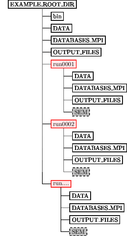
Figure 1.4 shows what the directory structure should looks like when simulating multiple earthquakes at ones.
-
The simulation is launched within the root directory
EXAMPLE_ROOT_DIR(usuallympirun -np N ./bin/xspecfem3D). -
DATAshould contain thePar_fileparameter file withNUMBER_OF_SIMULTANEOUS_RUNSas explained in Chapter [cha:Running-the-Mesher]. -
DATABASES_MPIand OUTPUT_FILES directory may contain the mesher output but they are not required as they are superseded by the ones in therunXXXdirectories. -
runXXXXdirectories must be created beforehand. There should be be as many asNUMBER_OF_SIMULTANEOUS_RUNSand the numbering should be contiguous, starting from0001. They all should haveDATA,DATABASES_MPIandOUTPUT_FILESdirectories. Additionally aSEMdirectory containing adjoint sources have to be created to perform adjoint simulations. -
runXXXX/DATAdirectories must all contain aCMTSOLUTIONfile, aSTATIONSfile along with an eventualSTATIONS_ADJOINTfile. -
If
BROADCAST_SAME_MESH_AND_MODELis set to.true.inDATA/Par_file, onlyrun0001/OUTPUT_FILESandrun0001/DATABASES_MPIdirectories need to contain the files outputted by the mesher. -
If
BROADCAST_SAME_MESH_AND_MODELis set to.false.inDATA/Par_file, everyrunXXXX/OUTPUT_FILESandrunXXXX/DATABASES_MPIdirectories need to contain the files outputted by the mesher. Note that while the meshes might have been created from different models and parameter sets, they should have been created using the same number of MPI processes.
References
Aki, K., and P. G. Richards. 1980. Quantitative Seismology, Theory and Methods. San Francisco, USA: W. H. Freeman.
Dahlen, F. A., and J. Tromp. 1998. Theoretical Global Seismology. Princeton, New-Jersey, USA: Princeton University Press.
Komatitsch, D., and J. Tromp. 2002. “Spectral-Element Simulations of Global Seismic Wave Propagation-I. Validation.” Geophys. J. Int. 149 (2): 390–412. https://doi.org/10.1046/j.1365-246X.2002.01653.x.
Meschede, M. A., C. L. Myhrvold, and J. Tromp. 2011. “Antipodal Focusing of Seismic Waves Due to Large Meteorite Impacts on Earth.” Geophys. J. Int. 187: 529–37.
This documentation has been automatically generated by pandoc based on the User manual (LaTeX version) in folder doc/USER_MANUAL/ (Dec 20, 2023)